API Documentation

Init file for pylim a package designed to work with measurement data for the radiation group at LIM author: Johannes Röttenbacher

bacardi

Functions to read in quicklook files and attitude correction

author: Johannes Röttenbacher

pylim.bacardi.fdw_attitude_correction(fdw, roll, pitch, yaw, sza, saa, fdir, r_off: float = 0, p_off: float = 0)

Attitude Correction for downward irradiance. Corrects downward irradiance for misalignment of the sensor (deviation from horizontal alignment).

• only direct fraction of irradiance can be corrected by the equation, therefore a direct fraction (fdir) has to be provided

• please check correct definition of the attitude angle

• for differences between the sensor attitude and the attitude given by an INS the offset angles (p_off and r_off) can be defined.

Parameters:

• fdw – downward irradiance [W m-2] or [W m-2 nm-1]

• roll – roll angle [deg] - defined positive for left wing up

• pitch – pitch angle [deg] - defined positive for nose down

• yaw – yaw angle [deg] - defined clockwise with North=0°

• sza – solar zenith angle [deg]

• saa – solar azimuth angle [deg] - defined clockwise with North=0°

• r_off – roll offset angle between INS and sensor [deg] - defined positive for left wing up

• p_off – pitch offset angle between INS and sensor [deg] - defined positive for nose down

• fdir – fraction of direct radiation [0..1] (0=pure diffuse, 1=pure direct)

Returns: corrected downward irradiance [W m-2] or [W m-2 nm-1] and correction factor

pylim.bacardi.read_bacardi_raw(filename: str, path: str) → Dataset

Read raw BACARDI data as provided by DLR

Parameters:

• filename – name of file

• path – path to file

Returns: Dataset with BACARDI data and time as dimension

bahamas

Functions to work with BAHAMAS data

• dictionary with plot properties for quicklook maps

• function to plot BAHAMAS map

• get position

• preprocess function for multiple file read in

• function to calculate distance between two bahamas samples

author: Johannes Röttenbacher

pylim.bahamas.calculate_distances(ds: Dataset) → Dataset

Calculate geodesic distance between each aircraft time step

Parameters:

ds – BAHAMAS dataset

Returns: New dataset with geodesic distances

pylim.bahamas.get_position(flight: str, timestamp: datetime | Timestamp) → Tuple[ndarray, ndarray, ndarray]

Given the flight and the exact time, get HALOs position.

Parameters:

• flight – Which flight to read in

• timestamp – exact time

Returns: latitude (deg), longitude (deg), altitude (m)

pylim.bahamas.plot_bahamas_flight_track(flight: str, **kwargs)

Plot a map of the flight track from BAHAMAS data with the location of HALO.

Parameters:

• flight – Flight name (eg. Flight_20210707a)

• **kwargs – outpath (str): where to save plot (default: bahamas_dir/plots)

Returns: Saves a png file

pylim.bahamas.preprocess_bahamas(ds: Dataset) → Dataset

Preprocessing function for xarray.read_mfdataset()

Returns: Dataset with dimension time

cirrus_hl

General information about the CIRRUS-HL campaign

• lookup dictionary to look up which spectrometer belongs to which inlet, which inlet is measuring up or downward irradiance and which filename part belongs to which channel

• dictionary relating flight with flight number

• BACARDI offsets

• dictionary which relates each measurement with the date of the transfer calibration for that measurement.

• take off and landing times according to BAHAMAS

• gopro local time and BAHAMAS time offset

• stop over locations for each double flight

• coordinates of airports

• radiosonde stations

• specific flight sections

• flight hours

• ozone files

author: Johannes Röttenbacher

ecrad

Functions translated from FORTRAN code in ecRad

author: Johannes Röttenbacher

pylim.ecrad.apply_ice_effective_radius(ds: Dataset) → Dataset

Apply ice effective radius function over a whole dataset

Parameters:

ds – IFS DataSet

Returns: DataSet with new variable re_ice containing the ice effective radius for each point

pylim.ecrad.apply_liquid_effective_radius(ds: Dataset) → Dataset

Apply liquid effective radius function over a whole dataset

Parameters:

ds – IFS DataSet

Returns: DataSet with new variable re_ice containing the ice effective radius for each point

pylim.ecrad.calc_ice_optics_baran2016(bands: str, ice_wp, qi, temperature)

Compute ice-particle scattering properties using a parameterization as a function of ice water mixing ratio and temperature.

From radiation_ice_optics_baran2016.F90 from the ecRad source code (https://github.com/ecmwf-ifs/ecrad).

3. Copyright 2016- ECMWF.

This software is licensed under the terms of the Apache Licence Version 2.0 which can be obtained at http://www.apache.org/licenses/LICENSE-2.0.

In applying this licence, ECMWF does not waive the privileges and immunities granted to it by virtue of its status as an intergovernmental organisation nor does it submit to any jurisdiction.

Author: Robin Hogan

Email: r.j.hogan@ecmwf.int

Modifications

2023-03-09 J. Röttenbacher Translated to python3

Parameters:

• bands – ‘sw’ or ‘lw’, shortwave or longwave bands

• ice_wp – Ice water path (kg m-2)

• qi – Mixing ratio (kg kg-1)

• temperature – Temperature (K)

Returns:

Total optical depth scat_od: Scattering optical depth g: Asymmetry factor

Return type:

od

pylim.ecrad.calc_ice_optics_baran2017(bands: str, ice_wp, qi, temperature)

Compute ice-particle scattering properties using a parameterization as a function of ice water mixing ratio and temperature.

From radiation_ice_optics_baran2017.F90 from the ecRad source code (https://github.com/ecmwf-ifs/ecrad).

3. Copyright 2017- ECMWF.

This software is licensed under the terms of the Apache Licence Version 2.0 which can be obtained at http://www.apache.org/licenses/LICENSE-2.0.

In applying this licence, ECMWF does not waive the privileges and immunities granted to it by virtue of its status as an intergovernmental organisation nor does it submit to any jurisdiction.

Author: Robin Hogan

Email: r.j.hogan@ecmwf.int

Modifications

2023-03-06 J. Röttenbacher Translated to python3

Parameters:

• bands – ‘sw’ or ‘lw’, shortwave or longwave bands

• ice_wp – Ice water path (kg m-2)

• qi – Mixing ratio (kg kg-1)

• temperature – Temperature (K)

Returns:

Total optical depth scat_od: Scattering optical depth g: Asymmetry factor

Return type:

od

pylim.ecrad.calc_ice_optics_fu_lw(ice_wp, r_eff)

Compute longwave ice-particle scattering properties using Fu et al. (1998) parameterization.

From radiation_ice_optics_fu.F90 from the ecRad source code (https://github.com/ecmwf-ifs/ecrad).

3. Copyright 2014- ECMWF.

This software is licensed under the terms of the Apache Licence Version 2.0 which can be obtained at http://www.apache.org/licenses/LICENSE-2.0.

In applying this licence, ECMWF does not waive the privileges and immunities granted to it by virtue of its status as an intergovernmental organisation nor does it submit to any jurisdiction.

Author: Robin Hogan

Email: r.j.hogan@ecmwf.int

Modifications

2020-08-10 R. Hogan Bounded r_eff to be <= 100um and g to be < 1.0

2023-03-06 J. Röttenbacher Translated to python3

Parameters:

• ice_wp – Ice water path (kg m-2)

• r_eff – Effective radius (m)

Returns:

Total optical depth scat_od: Scattering optical depth g: Asymmetry factor

Return type:

od

pylim.ecrad.calc_ice_optics_fu_sw(ice_wp, r_eff)

Compute shortwave ice-particle scattering properties using Fu (1996) parameterization. The asymmetry factor in band 14 goes larger than one for r_eff > 100.8 um, so we cap r_eff at 100 um. Asymmetry factor is capped at just less than 1 because if it is exactly 1 then delta-Eddington scaling leads to a zero scattering optical depth and then division by zero.

From radiation_ice_optics_fu.F90 from the ecRad source code (https://github.com/ecmwf-ifs/ecrad).

3. Copyright 2014- ECMWF.

This software is licensed under the terms of the Apache Licence Version 2.0 which can be obtained at http://www.apache.org/licenses/LICENSE-2.0.

In applying this licence, ECMWF does not waive the privileges and immunities granted to it by virtue of its status as an intergovernmental organisation nor does it submit to any jurisdiction.

Author: Robin Hogan

Email: r.j.hogan@ecmwf.int

Modifications

2020-08-10 R. Hogan Bounded r_eff to be <= 100um and g to be < 1.0

2023-03-06 J. Röttenbacher Translated to python3

Parameters:

• ice_wp – Ice water path (kg m-2)

• r_eff – Effective radius (m)

Returns:

Total optical depth scat_od: Scattering optical depth g: Asymmetry factor

Return type:

od

pylim.ecrad.calc_ice_optics_yi(bands: str, ice_wp, r_eff)

Compute shortwave ice-particle scattering properties using Yi et al. (2013) parameterization.

From radiation_ice_optics_yi.F90 from the ecRad source code (https://github.com/ecmwf-ifs/ecrad).

3. Copyright 2017- ECMWF.

This software is licensed under the terms of the Apache Licence Version 2.0 which can be obtained at http://www.apache.org/licenses/LICENSE-2.0.

In applying this licence, ECMWF does not waive the privileges and immunities granted to it by virtue of its status as an intergovernmental organisation nor does it submit to any jurisdiction.

Authors: Mark Fielding and Robin Hogan

Email: r.j.hogan@ecmwf.int

The reference for this ice optics parameterization is: Yi, B., P. Yang, B.A. Baum, T. L’Ecuyer, L. Oreopoulos, E.J. Mlawer, A.J. Heymsfield, and K. Liou, 2013: Influence of Ice Particle Surface Roughening on the Global Cloud Radiative Effect. J. Atmos. Sci., 70, 2794–2807, https://doi.org/10.1175/JAS-D-13-020.1

Modifications:

2023-03-06 J. Röttenbacher Translated to python3

Parameters:

• bands – ‘sw’ or ‘lw’, shortwave or longwave bands

• ice_wp – Ice water path (kg m-2)

• r_eff – effective radius (m)

Returns:

Total optical depth scat_od: Scattering optical depth g: Asymmetry factor

Return type:

od

pylim.ecrad.calc_pressure(ds: Dataset) → Dataset

Calculate the pressure at half and full hybrid model level. See https://confluence.ecmwf.int/display/CKB/ERA5%3A+compute+pressure+and+geopotential+on+model+levels%2C+geopotential+height+and+geometric+height

Parameters:

ds – DataSet as provided from the IFS output

Returns: DataSet with pressure at half and full model level

pylim.ecrad.calculate_pressure_height(ds: Dataset) → Dataset

Calculate the pressure height for the half and full model levels

Parameters:

ds – Dataset with temperature and pressure on model half and full levels (pressure_hl, temperature_hl, pressure_full, t)

Returns: Dataset with two new variables press_height_hl and press_height_full in meters

pylim.ecrad.cloud_overlap_decorr_len(latitude: float, scheme: int)

Implementation of the overlap decorrelation length parameter according to Shonk et al. 2010 (https://doi.org/10.1002/qj.647)

Parameters:

• latitude – Latitude of IFS grid cell

• scheme – Which scheme to apply?

Returns: decorr_len_edges_km, decorr_len_water_km, decorr_len_ratio

pylim.ecrad.get_input_version(version: str) → str

Return input version to given version string.

Parameters:

version – version string (e.g. v15.1)

Returns: Name of version

pylim.ecrad.get_model_level_of_altitude(altitude: DataArray, model_ds: Dataset, coord: str) → DataArray

Retrieve the model levels corresponding to a time series of altitude values such as given by a flight path.

Parameters:

• altitude – time series of altitude values in m, has to have the dimension time

• model_ds – model data set with index time, level and/or half_level and variables press_height_hl and/or press_height_full

• coord – which vertical coordinate to use for selection, either “half_level” or “level”

Returns:

pylim.ecrad.get_version_name(version: str) → str

Return version name to given version string.

Parameters:

version – Three character version string (e.g. v15)

Returns: Name of version

pylim.ecrad.ice_effective_radius(PPRESSURE, PTEMPERATURE, PCLOUD_FRAC, PQ_ICE, PQ_SNOW, PLAT)

From ice_effective_radius.F90 from the ecRad source code (https://github.com/ecmwf-ifs/ecrad).

3. Copyright 2016- ECMWF.

This software is licensed under the terms of the Apache Licence Version 2.0 which can be obtained at http://www.apache.org/licenses/LICENSE-2.0.

In applying this licence, ECMWF does not waive the privileges and immunities granted to it by virtue of its status as an intergovernmental organisation nor does it submit to any jurisdiction.

Purpose:

Calculate effective radius of ice clouds

Author:

Robin Hogan, ECMWF (using code extracted from radlswr.F90)

Original: 2016-02-24

Modifications:

2022-09-22 J. Röttenbacher translated Sun and Rikus part to python3

Ice effective radius = f(T,IWC) from Sun and Rikus (1999), revised by Sun (2001)

Parameters:

• PPRESSURE – (Pa)

• PTEMPERATURE –

• PCLOUD_FRAC – (kg/kg)

• PQ_ICE – (kg/kg)

• PQ_SNOW – (kg/kg)

• PLAT – (degrees)

Returns: ice effective radius in meter

pylim.ecrad.liquid_effective_radius(PPRESSURE, PTEMPERATURE, PCLOUD_FRAC, PQ_LIQ, PQ_RAIN)

From liquid_effective_radius.F90 from the ecRad source code (https://github.com/ecmwf-ifs/ecrad).

3. Copyright 2015- ECMWF.

This software is licensed under the terms of the Apache Licence Version 2.0 which can be obtained at http://www.apache.org/licenses/LICENSE-2.0.

In applying this licence, ECMWF does not waive the privileges and immunities granted to it by virtue of its status as an intergovernmental organisation nor does it submit to any jurisdiction.

Purpose:

Calculate effective radius of liquid clouds

Author:

Robin Hogan, ECMWF (using code extracted from radlswr.F90)

Original: 2015-09-24

Modifications:

2022-09-22 J. Röttenbacher translated Martin et al. (JAS 1994) part to python3

Parameters:

• PPRESSURE – (Pa)

• PTEMPERATURE –

• PCLOUD_FRAC – (kg/kg)

• PQ_LIQ – (kg/kg)

• PQ_RAIN – (kg/kg)

Returns: liquid effective radius in meter after Martin et al. (JAS 1994)

pylim.ecrad.make_ecrad_version_overview_csv(version_list: list = None, outpath: str = './docs/files') → None

Create a csv file with information on each version of the ecRad simulations

Parameters:

• version_list – list of versions of ecRad simulations e.g. [1, 3, 4, 5.2]

• outpath – path where csv file should be saved to

Returns: a csv file

halo_ac3

Background information and lookup dictionaries for the HALO-AC3 campaign

• dictionary to look up which spectrometer belongs to which inlet, which inlet is measuring up or downward irradiance and which filename part belongs to which channel.

• coordinates of airports and specific locations

• radiosonde stations

• flight names dictionary relates flight key to complete flight name

• dictionary which relates each measurement with the date of the transfer calibration for that measurement.

• take off and landing times

• gopro offsets from BAHAMAS time

• information on stabilization performance

• radiation square times

author: Johannes Röttenbacher

helpers

General helper functions and general information

author: Johannes Röttenbacher

pylim.helpers.cb_color_cycles

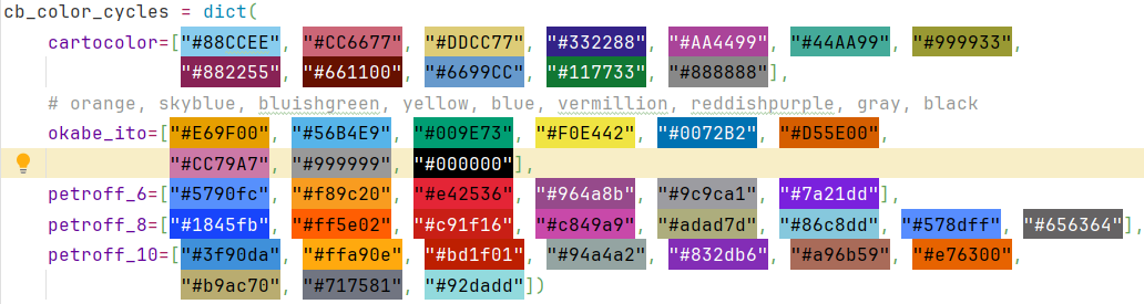
Colorblind friendly color cycles from the rcartocolor package, the Okabe-Ito palette [Color Universal Design (CUD) / Colorblind Barrier Free, n.d.] and the survey from Petroff [2021].

pylim.helpers.arg_nearest(array, value)

Find the index of the nearest value in an array.

Parameters:

• array – Input has to be convertible to an ndarray

• value – Value to search for

Returns: index of closest value

pylim.helpers.delete_folder_contents(folder: str) → None

Deletes all files and subfolders in a folder. From: https://stackoverflow.com/questions/185936/how-to-delete-the-contents-of-a-folder

Parameters:

folder – folder name or full path

Returns: nothing, but deletes all files in a folder

pylim.helpers.find_bases_tops(mask, rg_list)

This function finds cloud bases and tops for a provided binary cloud mask. :param mask: bool array containing False = signal, True=no-signal :type mask: np.array, dtype=bool :param rg_list: array of range values :type rg_list: np.ndarray

Returns:

list containing a dict for every time step consisting of cloud bases/top indices, range and width cloud_mask (np.array) : integer array, containing +1 for cloud tops, -1 for cloud bases and 0 for fill_value

Return type:

cloud_prop (list)

pylim.helpers.generate_specific_rows(filePath, userows=[])

Function for trajectory plotting

pylim.helpers.get_cb_friendly_colors(name: str = 'cartocolor') → list

Get colorblind friendly color cycle.

Parameters:

name – Name of color cycle

Returns: List with colorblind friendly colors

pylim.helpers.get_path(key: str, flight: str = None, campaign: str = 'cirrus-hl', instrument: str = None) → str

Read paths from the toml file according to the current working directory.

Parameters:

• key – which path to return, see config.toml for possible values

• flight – for which flight should the path be provided (e.g. Flight_20210625a for CIRRUS-HL or HALO-AC3_20220311_HALO_RF01 for HALO-AC3)

• campaign – campaign for which the paths should be generated

• instrument – if key=all which instrument to generate the path to? (e.g. BAHAMAS)

Returns: Path to specified data

pylim.helpers.hellinger_distance(p, q)

Compute the Hellinger distance between two probability distributions.

Parameters: p (numpy array): Probability distribution 1 (e.g., histogram). q (numpy array): Probability distribution 2 (e.g., histogram).

Returns: float: Hellinger distance between the two distributions.

Reference: - https://en.wikipedia.org/wiki/Hellinger_distance

pylim.helpers.longitude_values_for_gaussian_grid(latitudes: ~numpy.array, n_points: ~numpy.array, longitude_boundaries: ~numpy.array = None) -> (<built-in function array>, <built-in function array>)

Calculate the longitude values for each latitude circle on a reduced Gaussian grid. If the longitude boundaries are given only the longitude values within these boundaries are returned.

The ECMWF uses regular/reduced Gaussian grids to represent their model data. These have a fixed number of latitudes between the equator and each pole with either a regular amount of longitude points on each latitude ring or in case of a reduced Gaussian grid with a decreasing number of points towards the poles on each latitude ring. For more information on Gaussian grids as used by the ECMWF see: https://confluence.ecmwf.int/display/FCST/Gaussian+grids

When retrieving data on a reduced Gaussian grid the exact longitude values are not included in the data set and have to be calculated according to the definition of the grid. For this the latitude rings (latitudes) and the amount of longitude points on each latitude ring is needed (n_points). As one rarely retrieves the whole domain of the model the longitude boundaries are also needed to return the correct longitude values.

Parameters:

• latitudes – The latitude values of the Gaussian grid starting in the North

• n_points – The number of longitude points on each latitude circle (needs to be of same length as latitudes)

• longitude_boundaries – The longitude boundaries (E, W). E =-90, W =90, N=0, S=-180/180

Returns: Two arrays with repeating latitude values and the corresponding longitude values

pylim.helpers.make_dir(folder: str) → None

Creates folder if it doesn’t exist already.

Parameters:

folder – folder name or full path

Returns: nothing, but creates a new folder if possible

pylim.helpers.make_flag(boolean_array, name: str)

Make a list of flag values for plotting using a boolean array as input

Parameters:

• boolean_array – array like input with True and False

• name – replace True with this string

Returns: list with as many strings as there are True values in the input array

pylim.helpers.nested_dict_pairs_iterator(dict_obj: dict)

Loop over all values in a nested dictionary and return the key, value pair See: https://thispointer.com/python-how-to-iterate-over-nested-dictionary-dict-of-dicts/

Parameters:

dict_obj – nested dictionary

Returns: Each value in a nested dictionary with its key

pylim.helpers.nested_dict_values_iterator(dict_obj: dict)

Loop over all values in a nested dictionary See: https://thispointer.com/python-iterate-loop-over-all-nested-dictionary-values/

Parameters:

dict_obj – nested dictionary

Returns: Each value in a nested dictionary

pylim.helpers.read_command_line_args()

Read out command line arguments and save them to a dictionary. Expects arguments in the form key=value.

Returns: dictionary with command line arguments as dict[key] = value

pylim.helpers.set_cb_friendly_colors(name: str = 'cartocolor')

Set new colorblind friendly color cycle.

Parameters:

name – Name of color cycle

Returns: Modifies the standard pyplot color cycle

pylim.helpers.set_xticks_and_xlabels(ax: axis, time_extend: timedelta) → axis

This function sets the ticks and labels of the x-axis (only when the x-axis is time in UTC).

Options:

• time_extend > 7 days: major ticks every 2 day, minor ticks every 12 hours

• 7 days > time_extend > 2 days: major ticks every day, minor ticks every 6 hours

• 2 days > time_extend > 1 days: major ticks every 12 hours, minor ticks every 3 hours

• 1 days > time_extend > 12 hours: major ticks every 2 hours, minor ticks every 30 minutes

• 12hours > time_extend > 6 hours: major ticks every 1 hours, minor ticks every 30 minutes

• 6 hours > time_extend > 2 hour: major ticks every hour, minor ticks every 15 minutes

• 2 hours > time_extend > 30 min: major ticks every 15 minutes, minor ticks every 5 minutes

• 30 min > time_extend > 5 min: major ticks every 5 minutes, minor ticks every 1 minute

• else: major ticks every minute, minor ticks every 10 seconds

Parameters:

• ax – axis in which the x-ticks and labels have to be set

• time_extend – time difference of t_end - t_start (format datetime.timedelta)

Returns:

ax - axis with new ticks and labels

pylim.helpers.set_yticks_and_ylabels(ax: axis, time_extend: timedelta) → axis

This function sets the ticks and labels of the y-axis (only when the y-axis is time in UTC).

Options:

• time_extend > 7 days: major ticks every 2 day, minor ticks every 12 hours

• 7 days > time_extend > 2 days: major ticks every day, minor ticks every 6 hours

• 2 days > time_extend > 1 days: major ticks every 12 hours, minor ticks every 3 hours

• 1 days > time_extend > 12 hours: major ticks every 2 hours, minor ticks every 30 minutes

• 12hours > time_extend > 6 hours: major ticks every 1 hours, minor ticks every 30 minutes

• 6 hours > time_extend > 2 hour: major ticks every hour, minor ticks every 15 minutes

• 2 hours > time_extend > 15 min: major ticks every 15 minutes, minor ticks every 5 minutes

• 15 min > time_extend > 5 min: major ticks every 15 minutes, minor ticks every 5 minutes

• else: major ticks every minute, minor ticks every 10 seconds

Parameters:

• ax – axis in which the y-ticks and labels have to be set

• time_extend – time difference of t_end - t_start (format datetime.timedelta)

Returns:

ax - axis with new ticks and labels

pylim.helpers.setup_logging(dir: str, file: str = None, custom_string: str = None)

Setup up logging to file if script is called from console. If it is executed inside a console setup logging only to console.

Parameters:

• dir – Directory where to save logging file. Gets created if it doesn’t exist yet.

• file – Name of the file which called the function. Should be given via the __file__ attribute.

• custom_string – Custom String to append to logging file name. Logging file always starts with date and the name of the script being called.

Returns: Logger

pylim.helpers.strtobool(value)

Convert a string representation of a boolean value to a Python boolean.

Parameters:

value (str) – String representation of a boolean value.

Returns:

Python boolean value.

Return type:

bool

libradtran

Functions to process and plot libRadtran simulation files

author: Johannes Röttenbacher

pylim.libradtran.find_closest_radiosonde_station(latitude: float, longitude: float)

Given longitude and latitude, find the closest radiosonde station from the campaign dictionary

Parameters:

• latitude – in decimal degrees (N=positive)

• longitude – in decimal degrees (E=positive)

Returns: Name of the closest radiosonde station

pylim.libradtran.get_info_from_libradtran_input(filepath: str) → dict

Open a libRadtran input file and read out some information.

Parameters:

filepath – path to file

Returns: Some variables (latitude, longitude, time, header of output file, wavelength range, integrate flag)

pylim.libradtran.get_netcdf_global_attributes(campaign: str, flight: str, experiment: str)

Return a dictionary with globa attributes for a libRadtran simulation

Parameters:

• campaign – which campaign (cirrus-hl, halo-ac3)

• flight – which flight

• experiment – which experiment has been run

Returns: dictionary with global attributes

pylim.libradtran.get_netcdf_variable_attributes(solar_flag: bool, integrate_str: str, wavelength_str: str)

Return a dictionary with variable attributes for a libRadtran simulation

Parameters:

• solar_flag – whether the simulation was a solar or a terrestrial simulation

• integrate_str – whether the simulations was integrated at the end or not

• wavelength_str – wavelength range of the simulation

Returns: dictionary with variable attributes

pylim.libradtran.run_uvspec_parallel(input_files: list, uvspec_exe: str)

Run libRadtran simulations for all input files in parallel and check if an output has been created. Rerun the failed simulations a couple of times before quitting.

Parameters:

• input_files – list with full paths to each input file

• uvspec_exe – path to uvspec executable

Returns: Writes output and log files in directory of the input files

Raises: UsesWarning if a simulation fails more than 10 times

meteorological_formulas

General meteorological formulas

author: Johannes Röttenbacher

pylim.meteorological_formulas.barometric_height(pressure_profile, temperature_profile) → ndarray

Calculate the barometric height from a pressure and temperature profile.

\[\Delta h = \frac{\log\left(\frac{p(h_1)}{p(h_0)}\right) * R * T(h_1)}{M * g}\]

with \(h\) the height in meter, \(R\) the universal gas constant, \(T\) the temperature in Kelvin, \(M\) the molar mass of air and \(g\) earth’s acceleration.

Parameters:

• pressure_profile – pressure profile (Pa)

• temperature_profile – temperature profile (K)

Returns: barometric height (m)

@author: Hanno Müller, Johannes Röttenbacher

pylim.meteorological_formulas.barometric_height_simple(pressure)

Calculate the barometric height assuming a constant temperature of 0°C

Parameters:

pressure – pressure profile (Pa)

Returns: barometric_height

pylim.meteorological_formulas.calculate_absorption_coefficient_terrestrial(iwc: ArrayLike, reff: ArrayLike, density=916.7) → ArrayLike

Calculate the absorption coefficient (\(\beta_{abs}\)) of an ice cloud layer in the terrestrial wavelength range using the geometric optic assumption (ice particles are large compared to the incoming radiation) according to Eq. 7 in Francis et al. [1994]:

\[\beta_{abs} = \frac{3}{4} \frac{IWC}{\rho_{ice}r_{eff}}\]

with \(\rho_{ice}\) the density of ice and \(r_{eff}\) the ice effective radius according to Foot [1988].

Integrating this over altitude results in the optical depth of the ice cloud layer.

Parameters:

• iwc – Ice water content in kg/m^3

• reff – Ice effective radius in m

• density – Density of ice in kg/m^3

Returns: Absorption coefficient in m^-1 of the ice cloud layer in the solar wavelength range

pylim.meteorological_formulas.calculate_direct_sea_ice_albedo_ebert(cos_sza: float | DataArray)

Calculate the direct dry snow covered sea ice albedo for a specific solar zenith angle according to Ebert and Curry [1993].

Parameters:

cos_sza – Cosine of the solar zenith angle

Returns: direct albedo of dry snow covered sea ice

pylim.meteorological_formulas.calculate_extinction_coefficient_solar(iwc: ArrayLike, reff: ArrayLike, density=916.7) → ArrayLike

Calculate the extinction coefficient (\(\beta_{ext}\)) of an ice cloud layer in the solar wavelength range using the geometric optic assumption (ice particles are large compared to the incoming radiation) according to Eq. 10 in Francis et al. [1994]:

\[\beta_{ext} = \frac{3}{2} \frac{IWC}{\rho_{ice}r_{eff}}\]

with \(\rho_{ice}\) the density of ice and \(r_{eff}\) the ice effective radius according to Foot [1988].

Integrating this over altitude results in the optical depth of the ice cloud layer.

Parameters:

• iwc – Ice water content in kg/m^3

• reff – Ice effective radius in m

• density – Density of ice in kg/m^3

Returns: Extinction coefficient in m^-1 of the ice cloud layer in the solar wavelength range

pylim.meteorological_formulas.calculate_open_ocean_albedo_taylor(cos_sza: ArrayLike)

Calculate the open ocean albedo for direct incoming solar irradiance following Taylor et al. [1996].

\[\alpha = \frac{0.037}{1.1 * \cos(\theta)^{1.4} + 0.15}\]

with \(\theta\) being the solar zenith angle in radians.

Parameters:

cos_sza – cosine of the solar zenith angle

Returns: open ocean albedo

pylim.meteorological_formulas.relative_humidity_water_to_relative_humidity_ice(relative_humidity_water: float | ndarray | list, temperature: float | ndarray | list, version: str = 'huang')

Convert the relative humidity over water to relative humidity over ice using either the formulas by Huang [2018] or by Alduchov and Eskridge [1996].

\[RH_{ice} = \frac{RH_{water} * e_{s,w}}{e_{s,i}}\]

with \(e_{s,w}\) the saturation vapor pressure of water and \(e_{s,i}\) the saturation vapor pressure of ice:

\[ \begin{align}\begin{aligned}e_{s,w} = \frac{\exp\left(34.494 - \frac{4924.99}{t + 237.1}\right)}{(t + 105)^{1.157}} (t > 0°C)\\e_{s,i} = \frac{\exp\left(43.494 - \frac{6545.8}{t + 278}\right)}{(t + 868)^{2}} (t \le 0°C)\end{aligned}\end{align} \]

with \(t\) being the temperature in °C. When version is alduchov the following equations are used:

\[ \begin{align}\begin{aligned}e_{s,w} = 6.1094 * \exp\left(\frac{17.625 * t}{243.04 + t}\right)\\e_{s,i} = 6.1121 * \exp\left(\frac{22.587 * t}{273.86 + t}\right)\end{aligned}\end{align} \]

with \(t\) the temperature in °C.

Parameters:

• relative_humidity_water – ambient relative humidity in percent

• temperature – ambient temperature in °C

• version – which formulas to use for calculating the saturation vapor pressure of water and ice (‘huang’ or ‘alduchov’)

Returns: relative humidity over ice

reader

A collection of reader functions for instruments operated on HALO and model output files

author: Johannes Röttenbacher

pylim.reader.read_bacardi_raw(filename: str, path: str) → Dataset

Read raw BACARDI data as provided by DLR

Parameters:

• filename – name of file

• path – path to file

Returns: Dataset with BACARDI data and time as dimension

pylim.reader.read_bahamas(bahamas_path: str) → Dataset

Reader function for netcdf BAHAMAS data as provided by DLR.

Parameters:

bahamas_path – full path of netcdf file

Returns: xr.DataSet with BAHAMAS data and time as dimension

pylim.reader.read_cams_file(filepath: str) → Dataset

Read a CAMS atmosphere file

Parameters:

filepath – full path to nc file

Returns: DataSet with

pylim.reader.read_ecrad_output(filepath: str) → Dataset

Read in and preprocess a merged ecRad output file from :py:module:ecrad_merge_files.py

• Assign coordinates to dimensions

• Calculate pressure height in m

Parameters:

filepath – Full path to file

Returns: xarray DataSet with added coordinates to all dimensions of the file

pylim.reader.read_ins_gps_pos(filepath: str) → DataFrame

Read in a GPS position file as returned by the HALO-SMART INS system.

Parameters:

filepath – complete path to Nav_GPSPosxxxx.Asc file

Returns: time series with the GPS position data

pylim.reader.read_ins_gps_vel(filepath: str) → DataFrame

Read in a GPS velocity file as returned by the HALO-SMART INS system.

Parameters:

filepath – complete path to Nav_GPSVelxxxx.Asc file

Returns: time series with the GPS velocity data

pylim.reader.read_lamp_file(campaign: str = 'cirrus-hl', filename: str = None, plot: bool = True, save_fig: bool = True, save_file: bool = True) → DataFrame

Read in the 1000W lamp specification file interpolated to 1nm steps. Converts W/cm^2 to W/m^2.

Parameters:

• campaign – for which campaign should the lamp file be read in?

• filename – name of lamp file to be read in

• plot – plot lamp file?

• save_fig – save figure to standard plot path defined in config.toml?

• save_file – save lamp file to standard calib path deined in config.toml?

Returns: A data frame with the irradiance in W/m² and the corresponding wavelength in nm

pylim.reader.read_libradtran(flight: str, filename: str) → DataFrame

Read an old libRadtran simulation file generated by 01_dirdiff_BBR_Cirrus_HL_Server_jr.pro and add a DateTime Index.

Parameters:

• flight – which flight does the simulation belong to (e.g. Flight_20210629a)

• filename – filename

Returns: DataFrame with libRadtran output data

pylim.reader.read_nav_data(nav_path: str) → DataFrame

Reader function for Navigation data file from the INS used by the stabilization of SMART

Parameters:

nav_path – path to IMS file including filename

Returns: pandas DataFrame with headers and a DateTimeIndex

pylim.reader.read_ozone_sonde()

Reader function for ames formatted ozone sonde data from http://www.ndaccdemo.org/

Parameters:

filepath – complete path to file

Returns: pandas DataFrame with ozone volume mixing ratio

pylim.reader.read_pixel_to_wavelength(path: str, spectrometer: str) → DataFrame

Read file which maps each pixel to a certain wavelength for a specified spectrometer.

Parameters:

• path – Path where to find file

• spectrometer – For which spectrometer the pixel to wavelength mapping should be read in, refer to lookup table for possible spectrometers (e.g. ASP06_J3)

Returns: pandas DataFrame relating pixel number to wavelength

pylim.reader.read_smart_cor(path: str, filename: str) → DataFrame

Read dark current corrected SMART data files

Parameters:

• path – Path where to find file

• filename – Name of file

Returns: pandas DataFrame with column names and datetime index

pylim.reader.read_smart_raw(path: str, filename: str) → DataFrame

Read raw SMART data files

Parameters:

• path – Path where to find file

• filename – Name of file

Returns: pandas DataFrame with column names and datetime index

pylim.reader.read_stabbi_data(stabbi_path: str) → DataFrame

Read in stabilization platform data from SMART.

Parameters:

stabbi_path – full path to dat file

Returns: pandas DataFrame with headers and a DateTimeIndex

smart

These are functions in relation with the SMART instrument.

“_” denotes internal functions which are called inside other functions.

The functions are explained in their docstring and can be tested using the main frame. You can:

The reader functions were moved to pylim.reader.

• find the closest pixel and wavelength to any given wavelength for the given wavelength calibration file

• get information (date, measured property, channel) from the filename

• get the dark current for a specified measurement file with either option 1 or 2 and optionally plot it

• correct the raw measurement by the dark current

• plot the mean corrected measurement

• plot smart data either for one wavelength over time or for a range of or all wavelengths

• use the holoviews functions to create a dynamic map for interactive quicklooks in a jupyter notebook

author: Johannes Röttenbacher

pylim.smart.correct_smart_dark_current(flight: str, smart_file: str, option: int, **kwargs) → Series

Correct the raw SMART measurement for the dark current of the spectrometer. Only returns data when the shutter was open.

Parameters:

• flight – to which flight does the file belong to? (e.g. Flight_20210707a)

• smart_file – filename of file to correct

• option – which option should be used to get the dark current? Only relevant for channel “VNIR”.

• kwargs – path (str): path to file if not raw file path as given in config.toml, date (str): (yyyymmdd) date from which the dark current measurement should be used for VNIR (necessary if no transfer calibration was made on a measurement day) campaign (str): campaign to which smart file belongs to

Returns: Series with corrected smart measurement

pylim.smart.find_pixel(df: DataFrame, wavelength: 0.0) → Tuple[int, float]

Given the dataframe with the pixel to wavelength mapping, return the pixel and wavelength closest to the requested wavelength.

Parameters:

• df – Dataframe with column pixel and wavelength (from read_pixel_to_wavelength)

• wavelength – which wavelength are you interested in

Returns: closest pixel number and wavelength corresponding to the given wavelength

pylim.smart.get_dark_current(flight: str, filename: str, option: int, **kwargs) → Series | figure

Get the corresponding dark current for the specified measurement file to correct the raw SMART measurement.

Parameters:

• flight – to which flight does the file belong to? (e.g. Flight_20210707a)

• filename – filename (e.g. “2021_03_29_11_07.Fup_SWIR.dat”) of measurement file

• option – which option to use for VNIR (1, 2 or 3). Option 1: use measurements below 290 nm. Option 2: use dark measurements from transfer calibration (CIRRUS-HL folder structure expected). Option 3: use scaled dark current measurement from transfer calibration (HALO-AC3 folder structure expected).

• **kwargs – path (str): path to measurement file if not standard path from config.toml, plot (bool): show plot or not (default: True), date (str): yyyymmdd, date of transfer calibration with dark current measurement to use dark_filepath (str): complete path to dark current file to use campaign (str): campaign to which smart file belongs to

Returns: pandas Series with the mean dark current measurements over time for each pixel and optionally a plot of it

pylim.smart.get_info_from_filename(filename: str) → Tuple[str, str, str]

Using regular expressions some information from the filename is extracted.

Parameters:

filename – string in the form yyyy_mm_dd_hh_MM.[F/I][up/dw]_[SWIR/VNIR].dat (eg. “2021_03_29_11_07.Fup_SWIR.dat”)

Returns: A date string, the channel and the direction of measurement including the quantity.

pylim.smart.merge_vnir_swir_nc(vnir: Dataset, swir: Dataset) → Dataset

Merge the SMART nc files generated by smart_write_ncfile.py :param vnir: VNIR data set :param swir: SWIR data set

Returns: merged data set

pylim.smart.plot_calibrated_irradiance_flux(campaign: str, filename: str, wavelength: int | list | str, flight: str) → Overlay

Plot upward and downward irradiance as a time averaged series over the wavelength or as a time series for one wavelength. :param campaign: campaign name (cirrus-hl or halo-ac3) :param filename: Standard SMART filename :param wavelength: single or range of wavelength or “all” :param flight: flight folder (flight_xx)

Returns: holoviews overlay plot with two curves

pylim.smart.plot_complete_smart_spectra(path: str, campaign: str, filename: str, index: int, **kwargs) → None

Plot the complete spectra given by both channels from SMART calibrated measurement files for a given index (time step)

Parameters:

• path – where the file can be found

• campaign – campaign name (cirrus-hl or halo-ac3)

• filename – name of the file (standard SMART filename convention)

• index – which row to plot

• **kwargs – save_fig (bool): Save figure to plot path given in config.toml (default: False) plot_path (str): Where to save plot if not standard plot path

Returns: Shows and or saves a plot

pylim.smart.plot_complete_smart_spectra_interactive(path: str, campaign: str, filename: str, index: int) → Overlay

Plot the complete spectra given by both channels from SMART calibrated measurement files for a given index (time step) :param path: where the file can be found :param campaign: campaign name (cirrus-hl or halo-ac3) :param filename: name of the file (standard SMART filename convention) :param index: which row to plot

Returns: Shows and or saves a plot

pylim.smart.plot_mean_corrected_measurement(campaign: str, flight: str, filename: str, measurement: Series | list, measurement_cor: Series | list, option: int, **kwargs)

Plot the mean dark current corrected SMART measurement over time together with the raw measurement and the dark current.

Parameters:

• campaign – campaign name (cirrus-hl or halo-ac3)

• flight – to which flight does the file belong to? (e.g. Flight_20210707a)

• filename – name of file

• measurement – raw SMART measurements for each pixel averaged over time

• measurement_cor – corrected SMART measurements for each pixel averaged over time

• option – which option was used for VNIR correction

• **kwargs – save_fig (bool): save figure to current directory or just show it

Returns: plot

pylim.smart.plot_smart_data(campaign: str, flight: str, filename: str, wavelength: list | str, **kwargs) → axes

Plot SMART data in the given file. Either a time average over a range of wavelengths or all wavelengths, or a time series of one wavelength. Return an axes object to continue plotting or show it. TODO: add option to plot multiple files

Parameters:

• campaign – campaign name (cirrus-hl or halo-ac3)

• flight – to which flight does the file belong to? (e.g. Flight_20210707a)

• filename – Standard SMART filename

• wavelength – list with either one or two wavelengths in nm or ‘all’

• **kwargs – path (str): give path to filename if not default from config.toml, save_fig (bool): save figure? (default: False), plot_path (str): where to save figure (default: given in config.toml) ax (plt.axis): axes to already existing matplotlib axis

Returns: Shows a figure or saves it to disc.

pylim.smart.plot_smart_data_interactive(campaign: str, flight: str, filename: str, wavelength: list | str) → Curve

Plot SMART data in the given file. Either a time average over a range of wavelengths or all wavelengths, or a time series of one wavelength.

Parameters:

• campaign – campaign name (cirrus-hl or halo-ac3)

• flight – to which flight does the file belong to? (e.g. Flight_20210707a)

• filename – Standard SMART filename

• wavelength – list with either one or two wavelengths in nm or ‘all’

Returns: Creates an interactive figure

pylim.smart.plot_smart_ecrad_bands(smart: Dataset, bands: list, path: str = None, save_fig: bool = False)

Plot banded upward and downward irradiance for given ecRad bands

Parameters:

• smart – SMART data set containing variables fdn_banded and fup_banded

• bands – ecRad band numbers

• path – where to save figure to

• save_fig – whether to save figure

Returns: figure

pylim.smart.plot_smart_spectra(path: str, campaign: str, filename: str, index: int, **kwargs) → None

Plot a spectra from a SMART calibrated measurement file for a given index (time step)

Parameters:

• path – where the file can be found

• campaign – campaign name (cirrus-hl or halo-ac3)

• filename – name of the file (standard SMART filename convention)

• index – which row to plot

• **kwargs – save_fig (bool): Save figure to plot path given in config.toml (default: False), plot_path (str): Where to save plot if not standard plot path

Returns: Shows and or saves a plot

solar_position

Functions calculating the solar position

author: Hanno Müller, Johannes Röttenbacher

pylim.solar_position.dec(julian, year)

Declination calculated after Michalsky, J. 1988. Reference: Michalsky, J. 1988. The Astronomical Almanac’s algorithm for approximate solar position (1950-2050). Solar Energy 40 (3), pp. 227-235.

Parameters:

• julian – julian day (day of year) as calculated with julian2.pro

• year – The year (e.g., 2020)

Returns:

declination in (deg)

Examples

>>> dec(303, 2020)
-13.52916587749051

pylim.solar_position.get_saa(t0, lat, lon, year, month, day)

Calculates the solar azimuth angles. Requires function julian_day,local_time,dec :param t0: Time in UTC (in decimal hours, i.e. 10.5 for 10h30min) :param lat: Latitude (North positive) :param lon: Longitude (East positive) :param year: The year (e.g. 2020) :param month: The month (1-12) :param day: The day (1-31)

Returns:

The solar azimuth angle (deg)

Examples

>>> azimuth = get_saa(11, 51.34, 12.376, 2022, 2, 2)
>>> azimuth
173.75177751099122

pylim.solar_position.get_sza(t0, lat, lon, year, month, day, pres, temp)

Calculates the solar zenith angle Requires function julian_day,local_time,dec,refract

Copyright by Sebastian Schmidt

changes by Andre Ehrlich: - new declination parametrization after Michalsky, J. 1988. The Astronomical Almanac’s algorithm for approximate solar position (1950-2050). Solar Energy 40 (3), pp. 227-235. - refraction correction algorithm from Meeus,1991 - check: for SZA >95 no refraction correction

Parameters:

• t0 – Time in UTC (in decimal hours, i.e. 10.5 for 10h30min)

• lat – Latitude (North positive)

• lon – Longitude (East positive)

• year – The year (e.g. 2020)

• month – The month (1-12)

• day – The day (1-31)

• pres – Surface Pressure in hPa (for refraction correction)

• temp – Surface Temperature in deg C (for refraction correction)

Returns:

The solar zenith angle (deg)

pylim.solar_position.julian_day(year, month, day, t0)

Returns the day of the year (julian_day) for a given date. Jan 1 = 1, Feb 1 = 32 etc. Considers leap years and the time of day.

Parameters:

• year – The year (e.g. 2020)

• month – The month (1-12)

• day – The day (1-31)

• t0 – Time in UTC (dezimal hours)

Returns:

A value between 1 and 366, corresponding to the day of the year of year/month/day.

Examples

>>> jd = julian_day(2020, 2, 14, 6.8)
>>> jd
45.28333333333333

pylim.solar_position.local_time(julian, t0, lon)

Calculates the local solar time by accounting for - longitude - time equation (two versions are implemented, one commented, both are almost identical)

Parameters:

• julian – julian day (day of year) as calculated with julian2.pro

• t0 – Time in UTC (in decimal hours, i.e. 10.5 for 10h30min)

• lon – Longitude (East positive)

Returns:

Local solar time (in decimal hours, i.e. 10.5 for 10h30min)

Examples

>>> solar_local_time = local_time(265, 5.2, 14)
>>> solar_local_time
6.2521447402113886

pylim.solar_position.refract(elv, pres, temp)

Correction of the solar elevation angle for refraction Reference: J.Meeus, Astronomical Algorithms, 1991, pp102

Parameters:

• elv – solar elevation (rad)

• pres – station pressure (hPa)

• temp – station temperature (°C)

Returns:

corrected_elv = elv + refcor

Return type:

Refraction correction offset (rad) which needs to be applied after-wards

Examples

>>> refcor = refract(0.6, 850, 5)
>>> refcor
0.0003679487426608174